


Historical Background
Before the perceptron, AI was dominated by symbolic systems that manipulated logical rules such as:
IF Animal has feathers AND Animal flies
THEN Animal is Bird
These systems were powerful for structured problems but had a major weakness:
They couldn't learn from data.
Instead of manually programming knowledge into machines, perhaps machines could learn from experience.
Humans do not receive millions of IF-THEN rules at birth. Humans learn.
Researchers wanted machine that could improve automatically by observing examples rather than being explicitly programmed.
In 1943, Warren McCulloch and Walter Pitts proposed a simplified mathematical model of a biological neuron. Later, in 1958, Frank Rosenblatt developed the Perceptron, the first learning algorithm for such a neuron.
This was revolutionary because, instead of writing rules by hand, the machine could adjust itself based on examples.
Biological Inspiration
The perceptron was inspired by how biological neurons work.
The brain contains roughly: 86 Billions Neurons
Each neuron communicates with thousands of others.
A biological neuron consists of:
- Dendrites
- Receive signals
- Cell Body
- Processes signals
- Axon
- Sends signals to other neurons
- Synapses
- Connections between neurons.
Simplified:

Inputs
   ↓
[Dendrites]
   ↓
[Neuron]
   ↓
[Axon]
   ↓
Output

Scientists wondered:

Can we build a mathematical version of this process?
Biological process
- Thousands of neurons send signals.
- Some signals excite the neuron.
- Others inhibit it.
- The neuron sums all incoming signals.
- If the total exceeds a threshold, it “fires”
- Otherwise, it remains silent.
The perceptron imitates exactly this idea.
Mathematical Model
An artifical neuron receives inputs:
x1, x2, x3, ..... xnEach input has an associated weight:
w1, w2, w3, .... wnThe neuron computes:
z = (w1x1 + w2x2 + w3x3 + ... + wnxn) +  b

where:
xi = input
wi = weight (importance)
b = bias
z = weighted sum
This is called the weighted sum.
Understanding the Inputs
Imagine predicting whether someone likes coffee.
Features might be:
Age
Hours slept
Temperature
Stress level
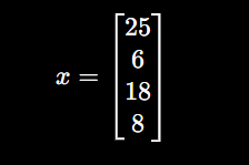
Suppose:
Age = 25
Sleep = 6
Temperature = 18
Stress = 8
Vector form:
What Are Weights
Wights determine the importance of each input.
Suppose
Age          0.1
Sleep       -0.8
Temperature  0.2
Stress       2
Interpretation: Higher weight means greater influence.
- Stress matters the most
- Sleep has a negative effect.
- Age matters little
- Temperature matters slightly.
The learning process adjusts these weights automatically. Learning is fundamentally the process of finding good weights.
Weighted Sum
Example:
Input	Weights
 2		 3
 5		 -2
 1		 4

Bias = 1
Compute:
z = 2 (3) + 5 (-2) + 1 (4) + 1
  = 6 -10 + 4 + 1
  = 1

This number (1) is not the final answer; it is the neuron's internal score.
Activation Function
After computing:
z = wx + bthe neuron applies an activation function.
General form:
output = activation(z)
The Step Function
The original perceptron uses the step function:
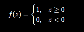
If the score is positive, output 1.
Otherwise, output 0.
This makes it suitable for binary decisions.
Example:
z = 5
Output = 1
z = -2
Output = 0This creates a hard yes/no decision.
Geometric Interpretation
This is where neural networks become interesting.
The perceptron creates a decision boundary.
In 2 dimensions:
w1x1 + w2x2 + b = 0defines a line.
Everything on one side; Class 1
Everything on other side; Class 0
The perceptron is therefore:
A linear classifier.
Decision Boundary
The perceptron partitions the input space into two regions.
Class A

xxxxxxxxxxxx
xxxxxxxxxxxx
xxxxxxxxxxxx

------------------------

oooooooooooo
oooooooooooo

Class B
The line separating the regions is the decision boundary.
Learning means moving this boundary until it separates the classes as well as possible.
Learning
The central question:
How do we find good weights?
The answer: Training
Initially, weights are random. Predictions are poor. Training adjusts the wreights to reduce errors.
Suppose:
Prediction = 0
Actual = 1
The model made a mistake.
We update weights.
General idea:
New Weight = Old Weight + CorrectionThis allows learning from errors.
The Perceptron Learning Rule
The original learning rule:
w = w + η(target - prediction)x

where:
η = learning rate
Learning rate determines update size.- If prediction = target
- No update occurs.
- If prediction != target
- Weights move in a better direction.
Training Process
Training follows a simple loop.
Initialize weights
 ↓
Predict
 ↓
Calculate Error
 ↓
Update Weights
 ↓
Repeat
What Can a Perceptron Learn
A single perceptron can learn linearly separably problems.
Examples:
- Spam vs. not spam
- Pass vs. fail
- Positive vs. negative sentiment
- Basic binary image classification
Example
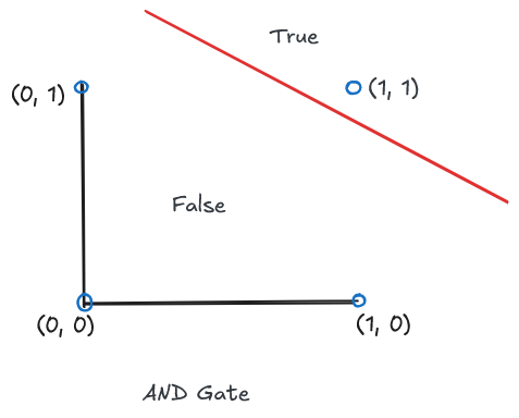
AND Gate
Inputs:
| x1 | x2 | Output |
|---|---|---|
| 0 | 0 | 0 |
| 0 | 1 | 0 |
| 1 | 0 | 0 |
| 1 | 1 | 1 |
The perceptron can learn this easily.
Decision boundary: Only output 1 when both inputs are 1.
OR Gate
Inputs:
| x1 | x2 | Output |
| 0 | 0 | 0 |
| 0 | 1 | 1 |
| 1 | 0 | 1 |
| 1 | 1 | 1 |
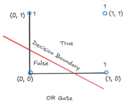
Also learnable.
The XOR Problem
Now consider:
| x1 | x2 | Output |
| 0 | 0 | 0 |
| 0 | 1 | 1 |
| 1 | 0 | 1 |
| 1 | 1 | 0 |
This is XOR.
Try drawing a single line that separates the classes.
Impossible.
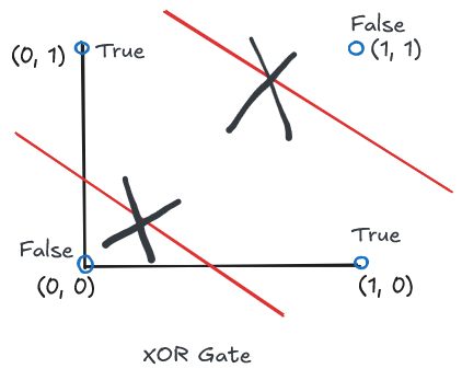
The XOR problem is not linearly separable. No single straight line can separate the two classes.
Therefore:
Single-Layer Perceptrons Cannot Solve XORThe Neural Network Crisis
In 1969: Marvin Minsky and Seymour Papert published: Perceptrons
They highlighted limitations of single-layer networks.
Funding disappeared. Neural network research nearly died.
This contributed heavily to the first AI winter.
Why XOR Changed Everything
XOR revealed something profound.
Intelligence requires:
Non-Linear Representations
A single neuron is not enough.
We need:
- Many Neurons
- Multiple Layers
This insight directly led to:
- Multi-Layer Perceptrons
and eventually:
Deep Learning

Join the discussion
Sign in with your account to post comments, reply to others, and participate in the conversation.
Login to Comment