What are the different types of data structure?

Data structures can be broadly classified into two types:

1. Linear: Linear data structures are those where data elements are arranged in a sequential (linear) manner. Example: Arrays, Linked List, Stacks, Queues, etc.
   • Linear means we can traverse them in a single run.
2. Non-linear: Non-linear data structures are those where data elements are not arranged in a sequential manner. They form a hierarchical or interconnected structure. Example: Trees, Graphs, etc.
   • Non-linear means we can't traverse them in a single run.

What is a Graph data structure?

A graph is a non-linear data structure consisting of nodes that have data and are connected to other nodes through edges. Graphs have a wide-ranging application in real life. These include analysis of electrical circuits, finding the shortest routes between two places, building navigation systems like Google Maps, even social media using graphs to store data about each user, etc.

A graph G(V, E) consists of:

• V: A set of vertices (also called nodes or points) where each vertex represents an entity.
• E: A set of edges (also called links or lines), which are connections between two vertices that show the relationship between them.

Example:

Let's consider a simple graph:

 A----B
 |   /|
 | /  |
 C----D

• Vertices: [A, B, C, D]
• Edges: [(A B), (A C), (B D), (B C), (C D)]

Graph Terminology

• Vertex (Node): A point or a node in a graph. Example: A, B, C, D.
• Edge (Link): A line connecting two vertices. Example: (A, B), (A, C).
• Adjacent Vertices: Two vertices are adjacent if they are connected by an edge.
• Degree: The number of edges connected to a vertex. In directed graphs, the degree is divided into in-degree (incoming edges) and out-degree (outgoing edges).
  • It is equivalent to 2*number of edges.
• Path: A sequence of edges that connect a sequence of vertices.
• Connected Graph: A graph where there is a path between every pair of vertices.
• Cycle: A path that starts and ends at the same vertex.

Types of Graphs

Graphs can be classified into several types based on their properties:

1️⃣ Directed vs Undirected Graphs (Based on Edge Direction)

Undirected Graph

In an undirected graph, edges do not have a direction. The connection between any two vertices goes both ways. It is bidirectional.

Example:

A -- B -- C
|    |
D -- E

In this graph, the edges are undirected, meaning an edge between A and B allows movement both from A to B and from B to A.

Edges have no direction, meaning if there is an edge between A and B, you can traverse both ways. Example: (A, B) means you can go from A to B and vice versa.

Directed Graph (Digraph):

In a directed graph, edges have a direction, meaning they only allow movement from one vertex to another in one direction.

Example:

A -> B -> C
|    ↑
↓    |
D    E

Here, the arrows show the direction of the edges. For example, you can go from A to B, but not from B to A unless there is a separate edge from B to A.

Edges have a direction. If there is an edge from A to B, you can only traverse from A to B. Example: A → B means you can only go from A to B, not the reverse.

2️⃣ Weighted vs Unweighted Graphs (Based on Edge Weight)

Weighted Graph:

A weighted graph assigns a weight (or cost) to each edge, representing the "cost" or "distance" of moving between vertices.

Example:

A --(3)--> B --(5)--> C
|           ↑
(2)         |
↓          (4)
D --(1)--> E

In this graph, each edge has a weight, such as 3 from A to B and 5 from B to C.

Edges have a weight or cost associated with them. This is useful in problems where you need to find the shortest path or minimum cost. Example: A → B (5) means the cost to go from A to B is 5.

• If weights are not assigned then we assume the unit (1) weights for every edges.

Unweighted Graph:

All edges have the same weight, often considered as 1.

3️⃣ Cyclic vs Acyclic Graphs (Based on Cycles)

Graphs can be classified on the basis of whether they contain cycles.

Cyclic Graph:

A cyclic graph contains at least one cycle. A cycle is a path of edges and vertices in which a vertex is reachable from itself by traversing the edges in the graph.

A cyclic graph contains at least one cycle, meaning you can start at a node and follow a path that leads back to the same node.

Example:

Example 3.a
Consider the following undireted graph:
1 --- 2
|     |
|     |
3 ----4

This graph contains a cycle (1->2->3->4)

Example 3.b
1-----2------3
      |      |
      |      |
      5------4
      |
      |
      6
This is also cyclic graph, as it contain atleast one cycle.

Acyclic Graph:

An acyclic graph is a graph that does not contain any cycles. That is, no vertex is reachable from itself by following the edges of the graph.

Example 3.c
1---2----3

Example 3.d
      1
     / \
    /   \
   2     3

4️⃣ Connected vs Disconnected Graphs (Based on Connectivity)

Connected Graph:

A connected graph is a graph in which there is a path between every pair of vertices. This means that starting from any vertex, it is possible to reach any other vertex by traversing the edges of the graph.

In undirected graphs, every pairs of vertices is connected by a path.

1 --- 2
|     |
3 --- 4

Disconnected Graph:

A disconnected graph is a graph in which there is at least one pair of vertices that are not connected by a path. In other words, the graph contains at least two separate components. Some vertices cannot be reached from others.

1 --- 2    3 --- 4

5️⃣ Other Special Types

Complete Graphs:

A complete graph is one in which every pair of vertices is connected by an edge.

A graph in which each vertex is connected to every other vertex.

Bipartite Graphs:

Vertices can be split into two disjoint sets such that every edge connects a vertex from one set to the other.

Trees:

A tree is a special kind of acyclic, connected graph. Trees are used in many hierarchical data representations.

Graph Representation ⬜

The two most commonly used representations for graphs are:

1. Adjacency Matrix
2. Adjacency Lists

1️⃣ Adjacency Matrix:

An adjacency matrix is a 2D array of size V x V, where V is the number of vertices in the graph. Each cell (i, j) in the matrix indicates whether there is an edge from vertex i to vertex j.

• Undirected Graph: The matrix will be symmetric.
• Directed Graph: The matrix may not be symmetric.

Example of an Adjacency Matrix:

A -- B
|    |
C -- D

The adjacency matrix representation:

   A B C D
A [0 1 1 0]
B [1 0 0 1]
C [1 0 0 1]
D [0 1 1 0]

Here, 1 represents the presence of an edge, and 0 indicates no edge.

How we store data in matrix:

1. Matrix Size: First of all, create a matrix of size n+1 x n+1 to accommodate vertex indexing from 0 to n.
2. Initialization: Initially our 2-D array will be filled with 0, indicating no edges between the vertices.
3. Adding Edges: When an edge (u, v) is added, we set matrix[u][v] and matrix[v][u] to 1 represent the undirected nature of the graph.
4. Weight Representation: Since weight are not provided in this scenario, we use 1 to indicate the presence of an edge.

#include <iostream>
#include <vector>

class Graph {
private:
    int vertices; // Number of vertices
    std::vector<std::vector<int>> adjMatrix; // Adjacency matrix

public:
    // Constructor
    Graph(int n) : vertices(n) {
        // Create an (n+1) x (n+1) adjacency matrix initialized to 0
        adjMatrix.resize(vertices + 1, std::vector<int>(vertices + 1, 0));
    }

    // Function to add an edge (for undirected graph)
    void addEdge(int u, int v) {
        adjMatrix[u][v] = 1; // Mark edge from u to v
        adjMatrix[v][u] = 1; // Mark edge from v to u (undirected)
    }

    // Function to print the adjacency matrix
    void printAdjMatrix() {
        for (int i = 0; i <= vertices; ++i) {
            for (int j = 0; j <= vertices; ++j) {
                std::cout << adjMatrix[i][j] << " ";
            }
            std::cout << std::endl;
        }
    }
};

int main() {
    int n = 3; // Example: Create a graph with 3 vertices (0 to 3)

    Graph g(n); // Create a graph instance

    g.addEdge(0, 2); // Add edge between 0 and 2
    g.addEdge(1, 2); // Add edge between 1 and 2
    g.addEdge(0, 1); // Add edge between 0 and 1

    std::cout << "Adjacency Matrix:" << std::endl;
    g.printAdjMatrix(); // Print the adjacency matrix

    return 0;
}

Code:

#include <bits/stdc++.h>
using namespace std;

int main() {  
    
    // Taking the input 
    int n, m;
    cin >> n >> m;
    
    // Adjacency matrix to store the graph
    int adj[n+1][n+1];
    
    // Add all the edges in the graph 
    for(int i = 0; i < m; i++) {
        // Taking the input
        int u, v;
        cin >> u >> v;
        
        // Adding the edges
        adj[u][v] = 1;
        
        /* This statement will be removed 
        in the case of directed graph */
        adj[v][u] = 1;
    }
    return 0;
}

Properties of the Adjacency Matrix:

1 Space Complexity: O(n^2)

• The space needed to represent a graph using its adjacency matrix is N² locations. It is a costly method as n² locations are consumed. It is preferred for dense graphs where the number of edges is more.
• Note: For directed graphs, if there is an edge between u and v it means the edge only goes from u to v, i.e., v is the neighbor of u, but vice versa is not true.

2 Edge Lookup:

• Checking if an edge exists between two vertices can be done in O(1) time since it only requires accessing the matrix at the specific indices.

3 Degree Calculation:

• For undirected graphs, the degree of a vertex can be calculated by summing the corresponding row (or column).
• For directed graphs, the out-degree can be calculated by summing the row, while the in-degree can be calculated by summing the column.

Disadvantage of using Adjacency Matrix:

While the edge look (checking if an edge exists between two vertices) is extremely fast in adjacency matrix representation however we have to reserve space for every possible link between all vertices, so it requires more space.

To Optimize it we can use Adjacency List

2️⃣ Adjacency List:

An adjacency list is an array of lists, where each list corresponds to a vertex and contains the vertices connected to it by an edge. This representation is more space-efficient for sparse graphs.

In C++, it is represented as the vector of integers:

vector<int> adj[n+1];

Example of an Adjacency List:

  0
 / \
1---2

The adjacency list representation:

0: {1 -> 2}
1: {0 -> 2}
2: {0 -> 1}

Code:

#include <bits/stdc++.h>
using namespace std;

int main() {
    
    // Taking the input
    int n, m;
    cin >> n >> m;
    
    // adjacency list for undirected graph
    vector<int> adj[n+1];
    
    // Add the edges to the list
    for(int i = 0; i < m; i++) {
        
        // Taking the input
        int u, v;
        cin >> u >> v;
        
        // Adding the edges
        adj[u].push_back(v);
        adj[v].push_back(u);
    }
    return 0;
}

OR

#include <iostream>
#include <vector>
#include <list>

class Graph {
private:
    int vertices; // Number of vertices
    std::vector<std::list<int>> adjList; // Adjacency list

public:
    // Constructor
    Graph(int n) : vertices(n) {
        // Initialize the adjacency list with empty lists
        adjList.resize(vertices);
    }

    // Function to add an edge (for undirected graph)
    void addEdge(int u, int v) {
        adjList[u].push_back(v); // Add v to the list of u
        adjList[v].push_back(u); // Add u to the list of v (undirected)
    }

    // Function to print the adjacency list
    void printAdjList() {
        for (int i = 0; i < vertices; ++i) {
            std::cout << i << ": ";
            for (const int &neighbor : adjList[i]) {
                std::cout << neighbor << " -> ";
            }
            std::cout << "NULL" << std::endl; // End of list
        }
    }
};

int main() {
    int n = 3; // Example: Create a graph with 3 vertices (0 to 2)

    Graph g(n); // Create a graph instance

    g.addEdge(0, 1); // Add edge between 0 and 1
    g.addEdge(1, 2); // Add edge between 1 and 2
    g.addEdge(0, 2); // Add edge between 0 and 2

    std::cout << "Adjacency List:" << std::endl;
    g.printAdjList(); // Print the adjacency list

    return 0;
}

Space Complexity: O(n + 2 * E)

The space needed to represent a graph using its adjacency matrix is N² locations. This representation is much better than the adjacency matrix for sparse graphs (where the number of edges is less), as matrix representation consumes n² locations, and most of them are unused.

In contrast, the adjacency list representation is more space-efficient for sparse graphs, as it only stores the existing edges. Thus its space complexity is O(n + 2*E), where n is node and E is edge.

Note: For directed graphs, if there is an edge between u and v it means the edge only goes from u to v, i.e., v is the neighbor of u, but vice versa is not true. Thus, The space needed to represent a directed graph using its adjacency list is E locations, where E denotes the number of edges, as here each edge data appears only once.

Note:

• vector<vector<int>>:
  • This is a dynamic 2D vector. Both the outer and inner vectors can be resized at runtime. It's ideal when the number of vertices (and consequently the number of rows) might change or isn't known at compile time.
• vector<int> adj[]:
  • This declares an array of vectors. The outer dimension (i.e., the number of vectors or “rows”) is fixed at compile time, while each inner vector remains dynamic. This representation works well when you know the number of vertices in advance.

Weighted Graph Representation:

Consider the following undirected weighted graph:

• For Adjacency matrix: the weight of the edge between node u and node v can be stored at the location a[u][v].

• For Adjacency list: Earlier in the adjacency list, a list of integers was stored in each index, but for weighted graphs, a list of pairs (adjacent node, edge weight) will be stored for each node using the following:

  vector<pair<int, int>> adjList[n+1];

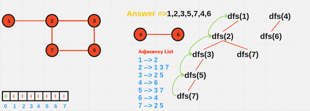
Connected Component in a Graph

A connected component in a graph is a group of nodes (subgraph) where:

1. All nodes in the group are connected to each other directly or through other nodes in that group.
2. No node in the group is connected to nodes outside of it.

Graph Traversal Algorithms

Graph traversal refers to the process of visiting (checking and/or updating) each vertex in a graph. Common traversal algorithms include:

1️⃣ Breadth-First Search (BFS)

BFS explores all vertices at the present depth level before moving on to the next level. It uses a queue data structure to explore the graph layer by layer.

BFS Algorithm:

1. Initialize:
   • Choose a starting node.
   • Create a queue to keep track of nodes to be visited.
   • Initialize a visited array to mark nodes that have already been processed.
2. Process the Starting Node:
   • Mark the starting node as visited.
   • Enqueue the starting node (add it to the back of the queue).
3. BFS Loop:
   • While the queue is not empty:
     1. Dequeue (remove from the front of the queue) the current node.
     2. For each unvisited neighbor of the current node:
        1. Mark the neighbor as visited.
        2. Enqueue the neighbor.
4. Repeat Until the Queue is Empty:
   • The BFS continues layer by layer, moving outward until all reachable nodes have been visited.

Code:

#include <iostream>
#include <vector>
#include <queue>

using namespace std;


void BFS(int start, vector<vector<int>>& adj, vector<bool>& visited) {
    queue<int> q;
    q.push(start);
    visited[start] = true;
    
    while (!q.empty()) {
        int node = q.front();
        q.pop();
        cout << node << " ";
        
        // Visit all unvisited neighbors
        for (int neighbor : adj[node]) {
            if (!visited[neighbor]) {
                visited[neighbor] = true;
                q.push(neighbor);
            }
        }
    }
}

int main() {
    int n = 5; // Number of nodes
    vector<vector<int>> adjList(n + 1);

    // Define edges
    adjList[1] = {2, 4};
    adjList[2] = {1, 3, 5};
    adjList[3] = {2};
    adjList[4] = {1, 5};
    adjList[5] = {2, 4};

    vector<bool> visited(n + 1, false);

    cout << "BFS starting from node 1:" << endl;
    BFS(1, adjList, visited);

    return 0;
}

// Output:
BFS starting from node 1:
1 2 4 3 5 

Complexity Analysis:

• Time Complexity: O(V + E), where V is the number of vertices (nodes) node E is the number of edges. Each node and edge is processed once.
• Space Complexity: O(V + E) + O(V) + O(V)
  • Adjacency List: O(V + E) We use adjacency list to store the graph. For a graph with V nodes and E edges, this takes O(V + E) space. Each node has a list of its neighbors, and each edge is stored once for undirected graphs or twice for directed graphs.
  • Visited Array: O(V) We use visited array to keep track of which nodes have been processed. This requires O(V) space, where V is the number of nodes (vertex).
  • Queue: O(V) In the worst case, all nodes might be added to the queue at once. Thus the queue can hold up to V nodes, requiring O(N) space.

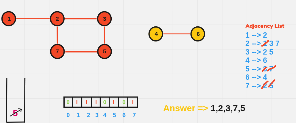
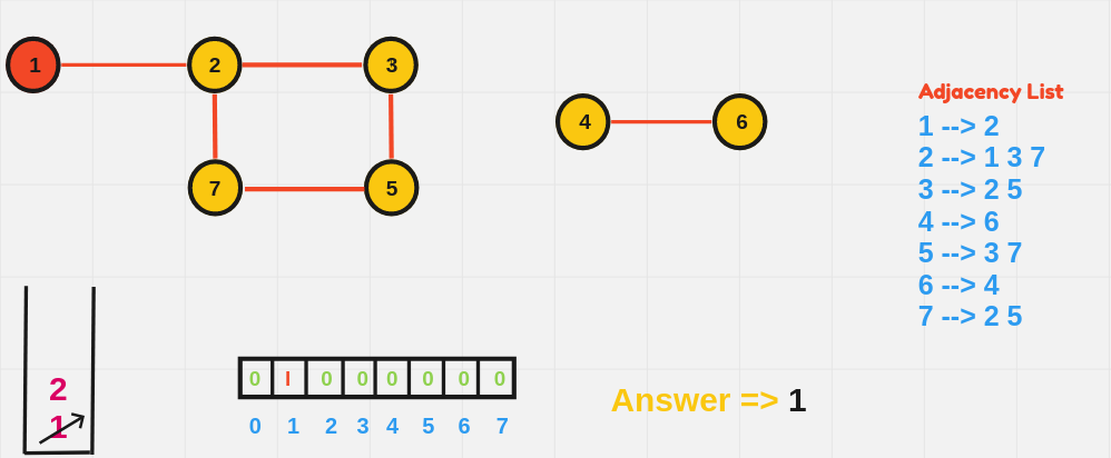
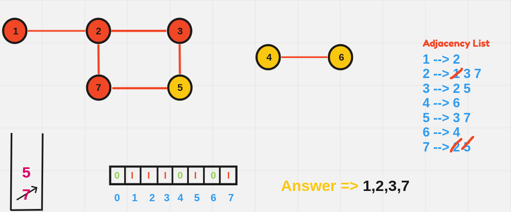
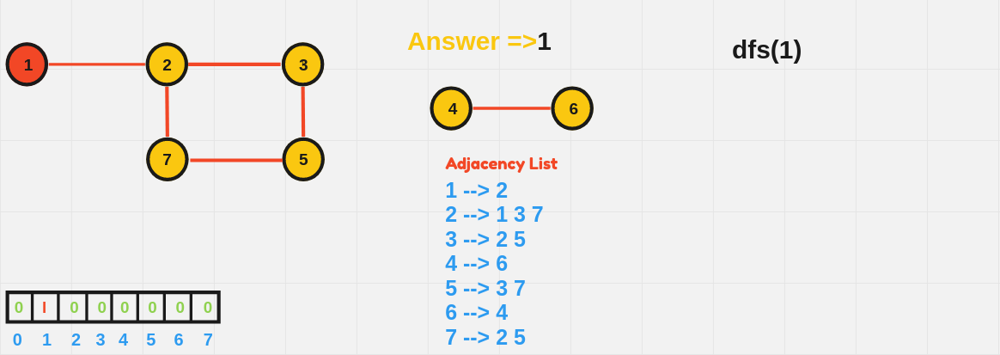
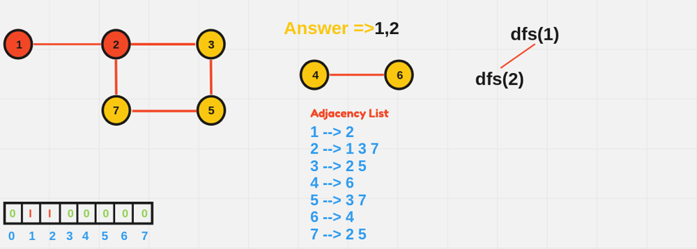
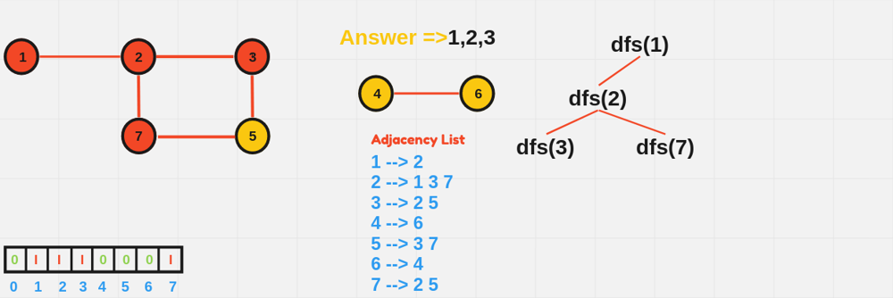
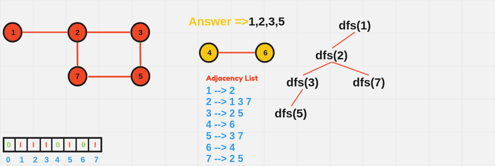
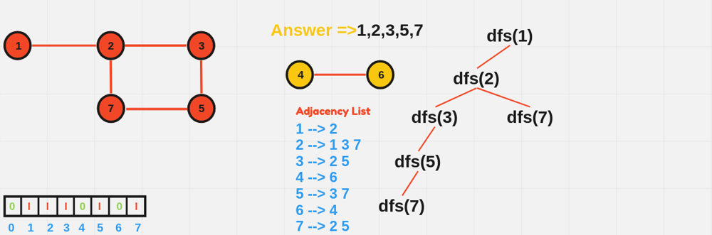
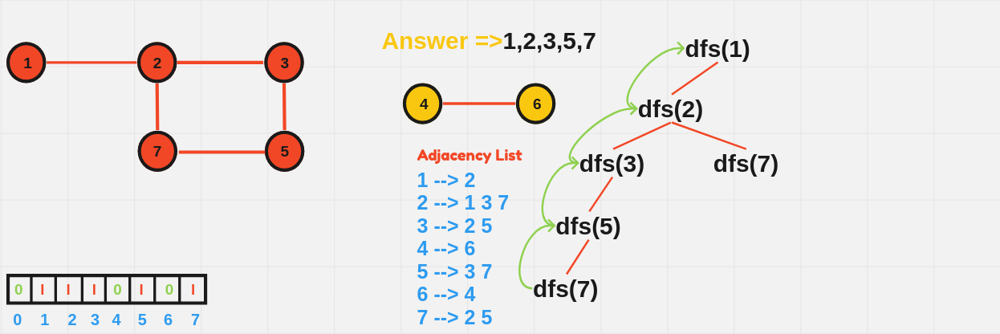
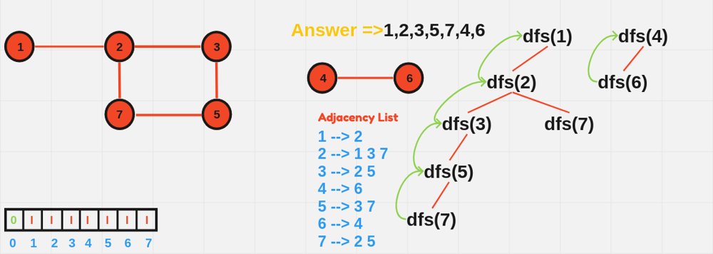
2️⃣ Depth-First Search (DFS)

DFS explores as far as possible along each branch before backtracking. It uses recursion (or an explicit stack) to visit vertices.

DFS Algorithm:

1. Initialize:
   • Start from a source node.
   • Use a visited array to keep track of nodes that have already been visited.
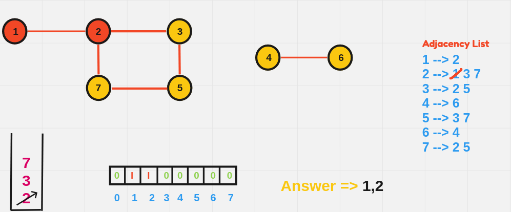
2. Explore Recursively or Iteratively:
   • For each unvisited neighbor of the current node:
     1. Mark the neighbor as visited.
     2. Move to that neighbor and repeat until there are no unvisited nodes to explore.
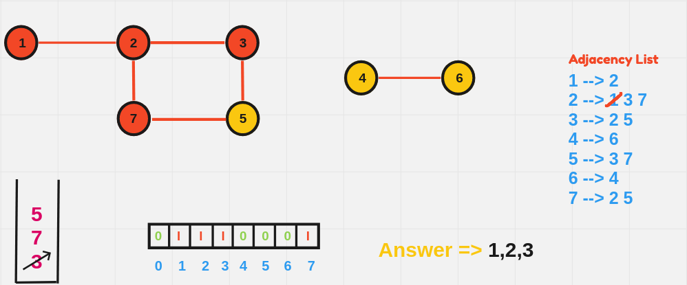
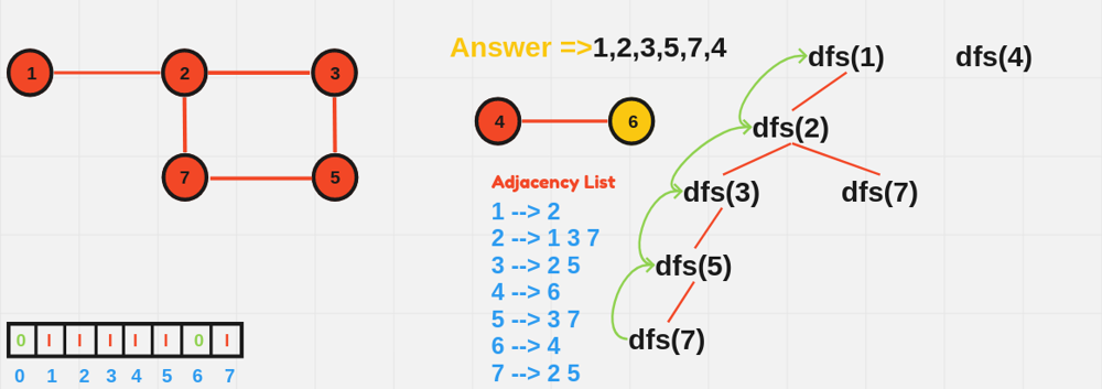
3. Backtrack:
   • Once you reach a node with no unvisited neighbors, backtrack to the previous node and continue exploring any remaining unvisited nodes.

Code:

With Recursion:

#include <iostream>
#include <vector>

using namespace std;

void DFS(int node, vector<vector<int>>& adj, vector<bool>& visited) {
    visited[node] = true;
    cout << node << " ";
    
    for (int neighbor : adj[node]) {
        if (!visited[neighbor]) {
            DFS(neighbor, adj, visited);
        }
    }
}


int main() {
    int n = 6; // Number of nodes
    vector<vector<int>> adjList(n + 1);

    // Define edges
    adjList[1] = {2, 3};
    adjList[2] = {1};
    adjList[3] = {1};
    adjList[4] = {5, 6};
    adjList[5] = {4};
    adjList[6] = {4};

    vector<bool> visited(n + 1, false);

    cout << "DFS starting from node 1:" << endl;
    DFS(1, adjList, visited);

    return 0;
}

With Explicit Stack:

#include <iostream>
#include <vector>
#include <stack>

void dfs(int start, std::vector<std::vector<int>>& adjList, std::vector<bool>& visited) {
    std::stack<int> s;
    s.push(start);

    while (!s.empty()) {
        int node = s.top();
        s.pop();

        if (!visited[node]) {
            visited[node] = true;
            std::cout << node << " ";

            // Push all unvisited neighbors onto the stack
            for (int neighbor : adjList[node]) {
                if (!visited[neighbor]) {
                    s.push(neighbor);
                }
            }
        }
    }
}

int main() {
    int n = 6; // Number of nodes
    std::vector<std::vector<int>> adjList(n + 1);

    // Define edges
    adjList[1] = {2, 3};
    adjList[2] = {1};
    adjList[3] = {1};
    adjList[4] = {5, 6};
    adjList[5] = {4};
    adjList[6] = {4};

    std::vector<bool> visited(n + 1, false);

    std::cout << "DFS starting from node 1:" << std::endl;
    dfs(1, adjList, visited);

    return 0;
}

Complexity Analysis:

• Time Complexity: O(V + E), where V is the number of vertices (nodes) and E is the number of edges. Each vertex and edge is processed once.
• Space Complexity: O(V)

Spanning Tree

A tree with n nodes and n-1 edges, and all nodes are reachable from each other.

A spanning tree is a subgraph that:

• Includes all n nodes.
• Contains exactly n-1 edges.
• Is connected and acyclic.

These three properties guarantee that the subgraph is a tree that “spans” the entire graph.

Examples:

Assume we are given an undirected graph with N nodes and M edges. Here, in the example, N=6 and M=7 as shown in the figure:

For the above graph, one of the spanning trees can be:

Another spanning trees are:

All the above spanning trees are subgraphs of the main graph, containing all the N nodes and N-1 edges to connect all nodes. For a particular spanning tree, the sum of edge weights of all its edges is called Weights of that spanning tree.

Note: A graph may have multiple spanning trees as shown in the above example.

Minimum Spanning Tree:

If the graph is weighted, a minimum spanning tree (MST) is a spanning tree with the smallest possible total edge weight.

Among all possible spanning trees of a graph, the minimum spanning tree is the one for which the sum of all the edge weights is the minimum.

The three spanning trees shown for the above graph have a weight of 18, 24 and 18 respectively. If all possible spanning trees are drawn, it will be found that the following spanning tree with the minimum sum of edge weights 16 is the minimum spanning tree for the above graph:

Note: A graph can have multiple minimum spanning trees.

Algorithms for finding the Minimum Spanning Tree for a given Graph?

There are two algorithms that come into picture when finding the Minimum Spanning Tree for a given graph:

• Prim's  Algorithm
• Krushkal Algorithm

References

1. https://leetcode.com/discuss/study-guide/2360573/become-master-in-graph